Map
The Map mark provides the following features:
- Plot a geographical map using various geo scales/projections
- Use ColorScale to create choropleths
- Support interactions like tooltips, selections etc.
Attributes
Data Attributes
Style Attributes
Let's look at examples of constructing maps using the pyplot API
pyplot
The function for plotting bar charts in pyplot is plt.geo. It takes one main argument:
- map_data Name of the map or json file required for the map data
Following map data are supported by default. For custom map data, a geo json file must be provided
| Map Data String | Description |
|---|---|
WorldMap |
World Map |
USStatesMap |
US States |
USCountiesMap |
US Counties |
EuropeMap |
Europe |
Tip
Panzoom is enabled by default. Click and drag on the white region surrounding the map to pan and use the mouse to zoom in and out. Double click on the white region to reset the map.
Code Examples
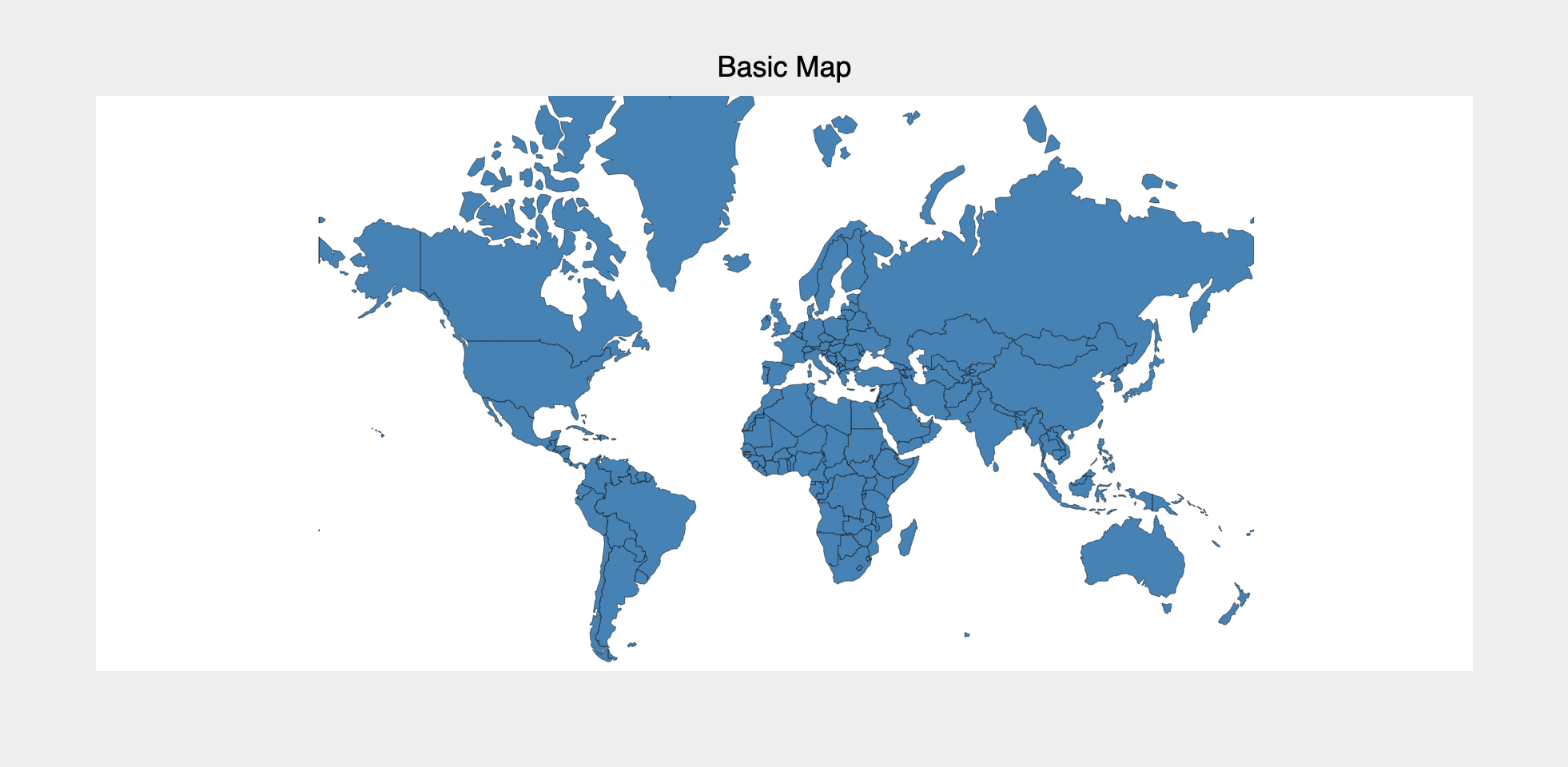
World Map
import bqplot.pyplot as plt

fig = plt.figure(title="World Map")
plt.geo(map_data="WorldMap",
        colors={"default_color": "steelblue"})
fig
Tip
Style attribute colors represents color of the items of the map when no color data is passed.
The dictionary should be indexed by the id of the element and have the corresponding colors as values.
The key default_color controls the items for which no color is specified.
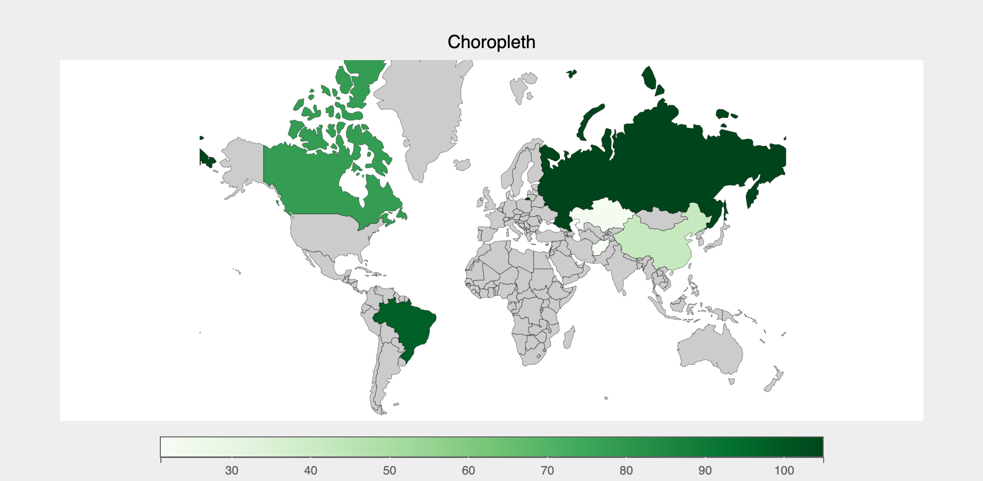
Choropleth
To render a choropleth, color data attribute needs to be passed. Note that color must be a dictionary whose keys are element ids
fig = plt.figure(title="Choropleth")

plt.scales(scales={"color": bq.ColorScale(scheme="Greens")})
chloro_map = plt.geo(
    map_data="WorldMap",
    color={643: 105, 4: 21, 398: 23, 156: 42, 124: 78, 76: 98},
    colors={"default_color": "Grey"},
)
fig
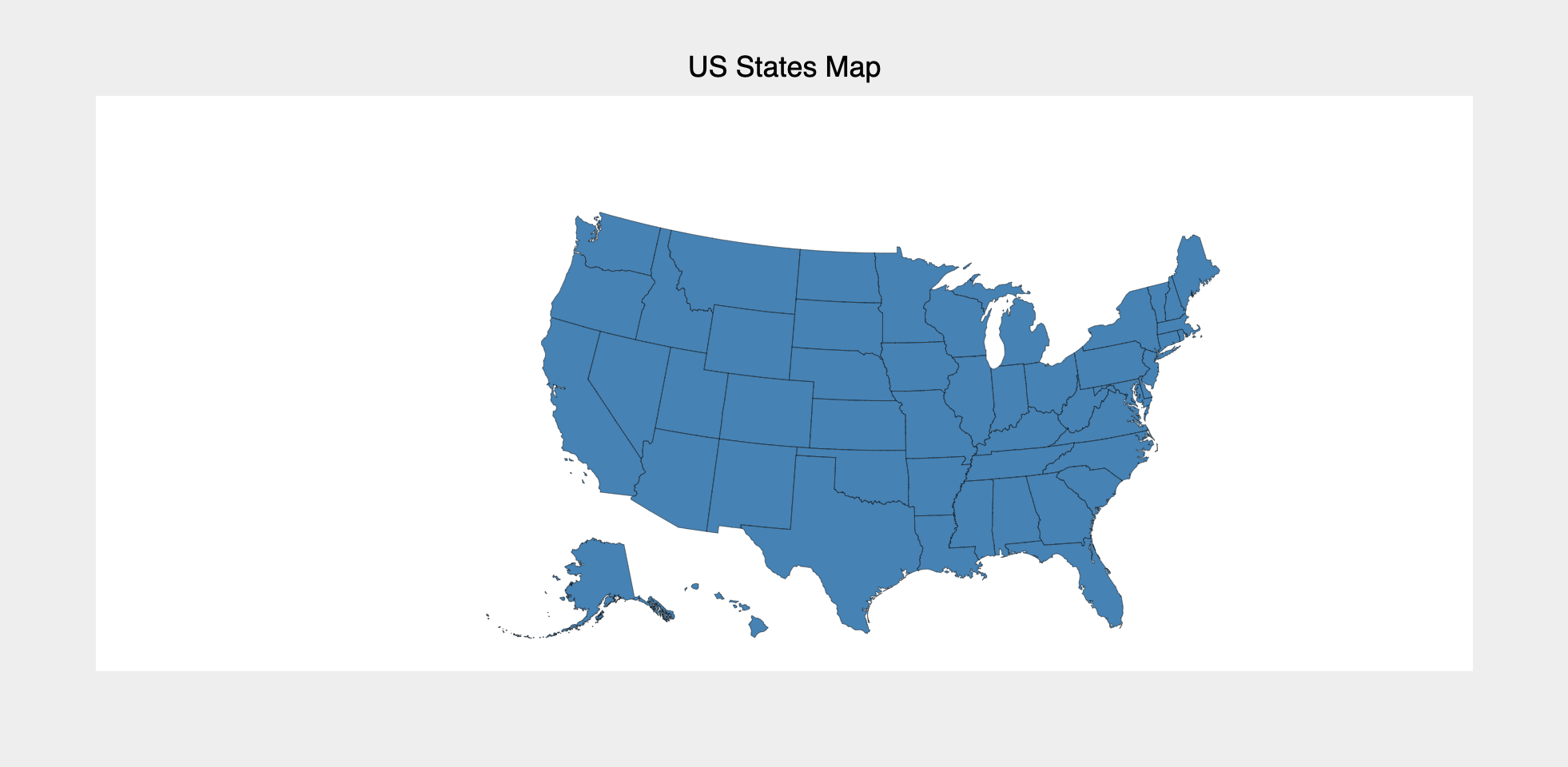
US Map
fig = plt.figure(title="US States Map")
plt.scales(scales={"projection": bq.AlbersUSA()})
states_map = plt.geo(map_data="USStatesMap", colors={"default_color": "steelblue"})
fig
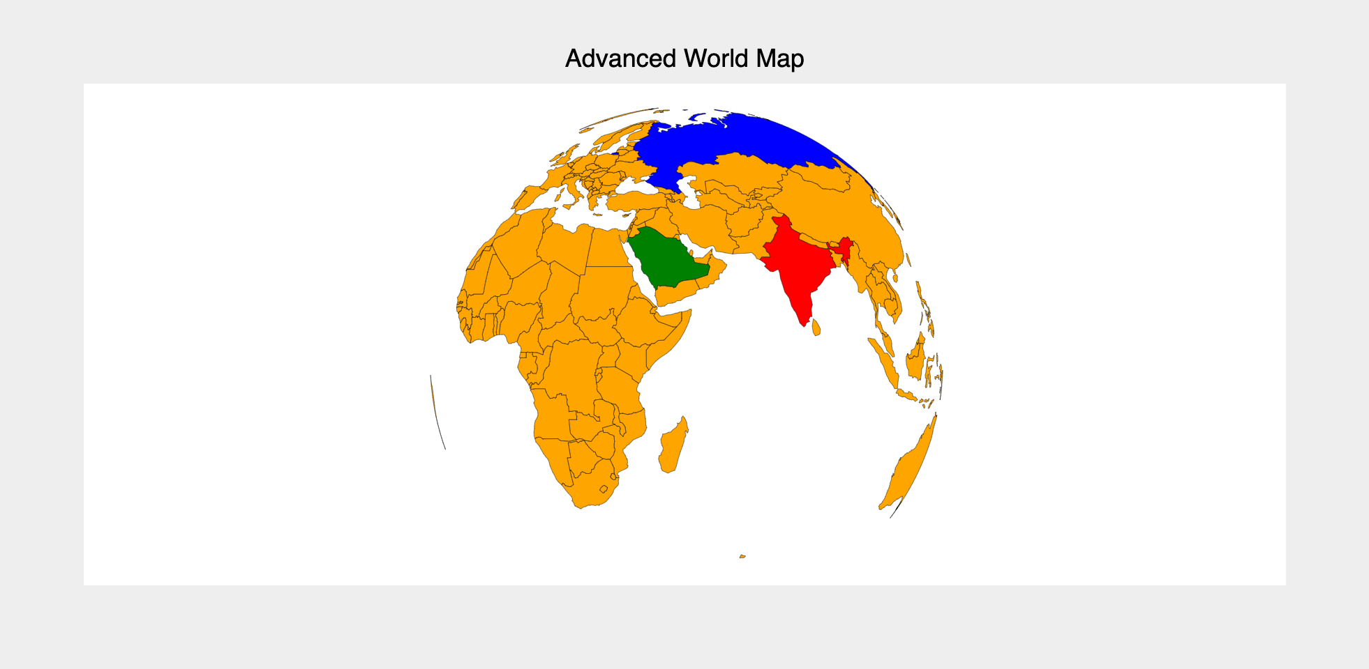
Advanced Projections
Use geo scale to customize the projections, like so:
import bqplot as bq

fig = plt.figure(title="Advanced World Map")
geo_scale = bq.Orthographic(scale_factor=375, center=[0, 25], rotate=(-50, 0))
plt.scales(scales={"projection": geo_scale})
map_mark = plt.geo(
    map_data="WorldMap",
    colors={682: "green", 356: "red", 643: "blue", "default_color": "orange"},
)
fig
Interactions
Tooltips
Tooltips can be added by setting the tooltip attribute to a Tooltip instance
fig = plt.figure(title="Interactions")
tooltip = bq.Tooltip(fields=["id", "name"])
map = plt.geo(
    map_data="WorldMap",
    tooltip=tooltip
)
fig
Selecting Map Element(s)
Map element(s) can be selected via mouse clicks. The selected attribute of the map mark will be automatically updated. Note that selected attribute is a list of ids of the selected elements.
Tip
Use the selected_style and unselected_style attributes (which are dicts) to apply CSS styling for selected and un-selected elements respectively
Callbacks can be registered on changes to selected attribute.
To select elements set interactions = {"click": "select"}. Single element can be selected by a mouse click. Mouse click + command key (mac) (or control key (windows)) lets you select multiple elements.
fig = plt.figure(title="World Map")
tooltip = bq.Tooltip(fields=["id", "name"])
map = plt.geo(
    map_data="WorldMap",
    tooltip=tooltip,
    interactions={"click": "select", "hover": "tooltip"}, # (1)!
)

# callback to invoke when elements are selected
def on_select(*args):
    selected_ids = map.selected
    if selected_ids is not None:
        # do something with selected elements
        print(selected_ids)

# register callback on selected attribute
map.observe(on_select, names=["selected"])

fig
- We have enabled both selections and tooltip here!
For an advanced example of maps and choropleths, checkout the Wealth Of Nations Choropleth dashboard in bqplot-gallery.
Example Notebooks
For detailed examples of maps, refer to the following example notebooks